
From OneR to Random Forests: A Decision Trees from Scratch Approach
Published on Jun 15, 2023 10:00 by KE Programmer
Table of Contents
1. Introduction
A decision trees from-scratch treatment for tabular data using the Identify Age-Related Conditions Kaggle competition.
We'll start with a very simple model, the OneR (One Rule) classifier, that makes predictions based on a single feature. We'll improve it step by step by performing splits on several features, implementing a decision tree, and finally combining many trees into a random forest.
2. Setup
Start by importing commonly used modules:
from fastai.imports import *
3. Data Processing
Get the dataset appropriately whether we're in Kaggle or not. If in Kaggle, it is assumed the competition dataset has been connected to the notebook.
import os
competition_name = "icr-identify-age-related-conditions"

is_kaggle = os.environ.get('KAGGLE_KERNEL_RUN_TYPE', '')
if is_kaggle:
    path = Path(f"/kaggle/input/{competition_name}")
else:
    import zipfile, kaggle
    path = Path.home() / '.kaggle' / 'input' / competition_name
    kaggle.api.competition_download_cli(competition_name, path=path.parent)
    zipfile.ZipFile(f'{path}.zip').extractall(path)
3.1. Load the Data
df_train = pd.read_csv(f'{path}/train.csv')
df_test = pd.read_csv(f'{path}/test.csv')
df_train.head()
             Id        AB          AF          AH  ...         GH         GI         GL  Class
0  000ff2bfdfe9  0.209377  3109.03329   85.200147  ...  22.136229  69.834944   0.120343      1
1  007255e47698  0.145282   978.76416   85.200147  ...  29.135430  32.131996  21.978000      0
2  013f2bd269f5  0.470030  2635.10654   85.200147  ...  28.022851  35.192676   0.196941      0
3  043ac50845d5  0.252107  3819.65177  120.201618  ...  39.948656  90.493248   0.155829      0
4  044fb8a146ec  0.380297  3733.04844   85.200147  ...  45.381316  36.262628   0.096614      1

[5 rows x 58 columns]
3.2. Explore the Data
df_train.describe()
               AB            AF           AH  ...          GI          GL       Class
count  617.000000    617.000000   617.000000  ...  617.000000  616.000000  617.000000
mean     0.477149   3502.013221   118.624513  ...   50.584437    8.530961    0.175041
std      0.468388   2300.322717   127.838950  ...   36.266251   10.327010    0.380310
min      0.081187    192.593280    85.200147  ...    0.897628    0.001129    0.000000
25%      0.252107   2197.345480    85.200147  ...   23.011684    0.124392    0.000000
50%      0.354659   3120.318960    85.200147  ...   41.007968    0.337827    0.000000
75%      0.559763   4361.637390   113.739540  ...   67.931664   21.978000    0.000000
max      6.161666  28688.187660  1910.123198  ...  191.194764   21.978000    1.000000

[8 rows x 56 columns]
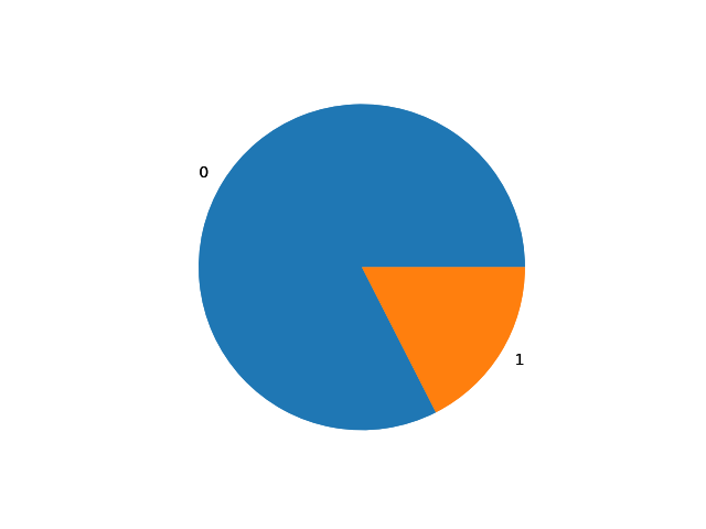
We can see that the mean of the dependent column Class is much
closer to zero than one. This means that observations with a positive
diagnosis are a smaller proportion of the training data. We can
confirm this by plotting a pie chart for column Class.
df_train.Class.value_counts().plot.pie()
We also check for null values:
df_train.isna().sum()
Id        0
AB        0
AF        0
AH        0
AM        0
AR        0
AX        0
AY        0
AZ        0
BC        0
BD        0
BN        0
BP        0
BQ       60
BR        0
BZ        0
CB        2
CC        3
CD        0
CF        0
CH        0
CL        0
CR        0
CS        0
CU        0
CW        0
DA        0
DE        0
DF        0
DH        0
DI        0
DL        0
DN        0
DU        1
DV        0
DY        0
EB        0
EE        0
EG        0
EH        0
EJ        0
EL       60
EP        0
EU        0
FC        1
FD        0
FE        0
FI        0
FL        1
FR        0
FS        2
GB        0
GE        0
GF        0
GH        0
GI        0
GL        1
Class     0
dtype: int64
df_train.info()
<class 'pandas.DataFrame'>
RangeIndex: 617 entries, 0 to 616
Data columns (total 58 columns):
 #   Column  Non-Null Count  Dtype
---  ------  --------------  -----
 0   Id      617 non-null    str
 1   AB      617 non-null    float64
 2   AF      617 non-null    float64
 3   AH      617 non-null    float64
 4   AM      617 non-null    float64
 5   AR      617 non-null    float64
 6   AX      617 non-null    float64
 7   AY      617 non-null    float64
 8   AZ      617 non-null    float64
 9   BC      617 non-null    float64
 10  BD      617 non-null    float64
 11  BN      617 non-null    float64
 12  BP      617 non-null    float64
 13  BQ      557 non-null    float64
 14  BR      617 non-null    float64
 15  BZ      617 non-null    float64
 16  CB      615 non-null    float64
 17  CC      614 non-null    float64
 18  CD      617 non-null    float64
 19  CF      617 non-null    float64
 20  CH      617 non-null    float64
 21  CL      617 non-null    float64
 22  CR      617 non-null    float64
 23  CS      617 non-null    float64
 24  CU      617 non-null    float64
 25  CW      617 non-null    float64
 26  DA      617 non-null    float64
 27  DE      617 non-null    float64
 28  DF      617 non-null    float64
 29  DH      617 non-null    float64
 30  DI      617 non-null    float64
 31  DL      617 non-null    float64
 32  DN      617 non-null    float64
 33  DU      616 non-null    float64
 34  DV      617 non-null    float64
 35  DY      617 non-null    float64
 36  EB      617 non-null    float64
 37  EE      617 non-null    float64
 38  EG      617 non-null    float64
 39  EH      617 non-null    float64
 40  EJ      617 non-null    str
 41  EL      557 non-null    float64
 42  EP      617 non-null    float64
 43  EU      617 non-null    float64
 44  FC      616 non-null    float64
 45  FD      617 non-null    float64
 46  FE      617 non-null    float64
 47  FI      617 non-null    float64
 48  FL      616 non-null    float64
 49  FR      617 non-null    float64
 50  FS      615 non-null    float64
 51  GB      617 non-null    float64
 52  GE      617 non-null    float64
 53  GF      617 non-null    float64
 54  GH      617 non-null    float64
 55  GI      617 non-null    float64
 56  GL      616 non-null    float64
 57  Class   617 non-null    int64
dtypes: float64(55), int64(1), str(2)
memory usage: 279.7 KB
3.3. Data Cleaning
On the competition's data tab, we're informed that all columns are
numeric with the exception of EJ, which is categorical. We'll
replace null values with modes, and convert EJ to a pandas
categorical column.
modes = df_train.mode().iloc[0]
def process_data(df):
    df.fillna(modes, inplace=True)
    df["EJ"] = pd.Categorical(df.EJ)

process_data(df_train)
process_data(df_test)
df_train.info()
<class 'pandas.DataFrame'>
RangeIndex: 617 entries, 0 to 616
Data columns (total 58 columns):
 #   Column  Non-Null Count  Dtype
---  ------  --------------  -----
 0   Id      617 non-null    str
 1   AB      617 non-null    float64
 2   AF      617 non-null    float64
 3   AH      617 non-null    float64
 4   AM      617 non-null    float64
 5   AR      617 non-null    float64
 6   AX      617 non-null    float64
 7   AY      617 non-null    float64
 8   AZ      617 non-null    float64
 9   BC      617 non-null    float64
 10  BD      617 non-null    float64
 11  BN      617 non-null    float64
 12  BP      617 non-null    float64
 13  BQ      617 non-null    float64
 14  BR      617 non-null    float64
 15  BZ      617 non-null    float64
 16  CB      617 non-null    float64
 17  CC      617 non-null    float64
 18  CD      617 non-null    float64
 19  CF      617 non-null    float64
 20  CH      617 non-null    float64
 21  CL      617 non-null    float64
 22  CR      617 non-null    float64
 23  CS      617 non-null    float64
 24  CU      617 non-null    float64
 25  CW      617 non-null    float64
 26  DA      617 non-null    float64
 27  DE      617 non-null    float64
 28  DF      617 non-null    float64
 29  DH      617 non-null    float64
 30  DI      617 non-null    float64
 31  DL      617 non-null    float64
 32  DN      617 non-null    float64
 33  DU      617 non-null    float64
 34  DV      617 non-null    float64
 35  DY      617 non-null    float64
 36  EB      617 non-null    float64
 37  EE      617 non-null    float64
 38  EG      617 non-null    float64
 39  EH      617 non-null    float64
 40  EJ      617 non-null    category
 41  EL      617 non-null    float64
 42  EP      617 non-null    float64
 43  EU      617 non-null    float64
 44  FC      617 non-null    float64
 45  FD      617 non-null    float64
 46  FE      617 non-null    float64
 47  FI      617 non-null    float64
 48  FL      617 non-null    float64
 49  FR      617 non-null    float64
 50  FS      617 non-null    float64
 51  GB      617 non-null    float64
 52  GE      617 non-null    float64
 53  GF      617 non-null    float64
 54  GH      617 non-null    float64
 55  GI      617 non-null    float64
 56  GL      617 non-null    float64
 57  Class   617 non-null    int64
dtypes: category(1), float64(55), int64(1), str(1)
memory usage: 275.5 KB
EJ now has a category column type.
A decision tree only requires that the column values can be ordered
numerically. For the categorical column EJ, we'll use the underlying
categorical codes as its values.
df_train.EJ.head()
0    B
1    A
2    B
3    B
4    B
Name: EJ, dtype: category
Categories (2, str): ['A', 'B']
df_train.EJ.cat.codes.head()
0    1
1    0
2    1
3    1
4    1
dtype: int8
Segregate the categorical, numeric and dependent variables:
categoricals = ["EJ"]
dependent = "Class"
conts = [column for column in df_train.columns
         if not column in categoricals + [dependent] + ["Id"]]
4. Binary Splits
A decision tree is built on binary splits, i.e. using the value of a column
to split the rows into two groups. Let's use a barplot and countplot to
analyse how splitting on EJ relates to the diagnosed class.
import seaborn as sns

fig, axs = plt.subplots(1, 2, figsize=(11, 5))
sns.barplot(data=df_train, y=dependent, x="EJ", ax=axs[0])\
    .set(title="Positive Diagnosis Rate")
sns.countplot(data=df_train, x="EJ", ax=axs[1])\
    .set(title="Histogram")
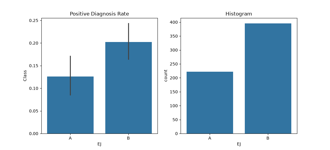
We have a higher positivity rate for category B (~20%) than category A (~13%). We also have a much higher proportion of observations with category B (~400) than category A (~230).
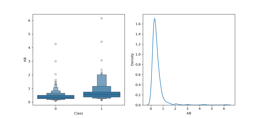
We can also do a split based on a continuous column. We'll go with column
AB just for demonstration. We use a boxplot to compare the averages of
both positive and negative diagnosis based on the trait AB and a density
plot to visualize the distribution of observations on AB.
fig, (ax1, ax2) = plt.subplots(nrows=1, ncols=2, figsize=(11, 5))
sns.boxenplot(data=df_train, x=dependent, y="AB", ax=ax1)
sns.kdeplot(data=df_train, x="AB", ax=ax2)
4.1. The Score Function
Since we have a large number of columns, it would be tedious to plot each of them and figure out how well it partitions between positive and negative diagnosis. We can create a function that helps us quickly evaluate different splits by calculating a measure of impurity.
The key idea in determining a good split is that the it the dependent variable is as homogenous as possible within each group.
The lower the standard deviation of the dependent variable in a group, the more homogenous it is.
Next we multiple the std deviation with the group size, so that a larger group contributes more to the score, before normalizing the score using the total number of observations.
def score(col, y, split_value):
    lhs = col <= split_value
    return (_side_score(lhs, y) + _side_score(~lhs, y))/len(y)

def _side_score(side, y):
    count = side.sum()
    if count <=1: return 0
    return y[side].std() * count
For instance, the score based on value 0.5 for column AB:
score(df_train.AB, df_train[dependent], 0.5)
0.36017711175753037
For the categorical column, we'd need to replace the column string values with their underlying codes:
df_train_n = df_train.copy()
df_train_n[categoricals] = df_train_n[categoricals].apply(lambda x: x.cat.codes)
df_train_n[categoricals].head()
   EJ
0   1
1   0
2   1
3   1
4   1
We then calculate the score using <= 1 as our split:
score(df_train_n.EJ, df_train_n[dependent], 1)
0.3803100751041243
4.2. Finding the Best Split
To help us find the best split point, we'll iterate through the columns, and for each, we iterate through its unique values to find the best split point for the column.
For example, to find the best split point for column AB:
col = df_train_n["AB"]
y = df_train_n[dependent]
uniques = col.unique()
uniques.sort()
uniques[:50]
array([0.081187 , 0.08546  , 0.098279 , 0.102552 , 0.111098 , 0.119644 ,
       0.1217805, 0.1303265, 0.132463 , 0.136736 , 0.141009 , 0.145282 ,
       0.149555 , 0.153828 , 0.1559645, 0.158101 , 0.1602375, 0.162374 ,
       0.166647 , 0.17092  , 0.175193 , 0.179466 , 0.183739 , 0.1858755,
       0.188012 , 0.1901485, 0.192285 , 0.196558 , 0.200831 , 0.2029675,
       0.205104 , 0.209377 , 0.21365  , 0.217923 , 0.222196 , 0.2243325,
       0.226469 , 0.230742 , 0.235015 , 0.239288 , 0.243561 , 0.247834 ,
       0.252107 , 0.25638  , 0.260653 , 0.2627895, 0.264926 , 0.269199 ,
       0.2713355, 0.273472 ])
Get the best split for AB:
scores = np.array([score(col, y, split) for split in uniques])
uniques[scores.argmin()]
0.410208
Create a function that gets the best split for for any column:
def min_column(df, col_name):
    col, y = df[col_name], df[dependent]
    uniques = col.unique()
    scores = np.array([score(col, y, split) for split in uniques])
    index = scores.argmin()
    return uniques[index], scores[index]
min_column(df_train_n, "AB")
We then try the same for the categorical variable:
min_column(df_train_n, "EJ")
| np.int8 | (0) | np.float64 | (0.3773339803468088) |
We then calculate the best split points for each of the columns to find the best split overall:
columns = conts + categoricals
splits = {col: min_column(df_train_n, col) for col in columns}
splits
{'AB': (np.float64(0.410208), np.float64(0.3561906829723693)), 'AF': (np.float64(2808.64232), np.float64(0.35583548065304915)), 'AH': (np.float64(193.801377), np.float64(0.3761985927636321)), 'AM': (np.float64(149.318758), np.float64(0.367338331639673)), 'AR': (np.float64(16.327194), np.float64(0.3678281215243884)), 'AX': (np.float64(17.877462), np.float64(0.37677322461475915)), 'AY': (np.float64(0.6019965), np.float64(0.37677322461475915)), 'AZ': (np.float64(10.971782), np.float64(0.3782810033906922)), 'BC': (np.float64(13.500788), np.float64(0.35968813799570454)), 'BD ': (np.float64(12083.34891), np.float64(0.3749922782916859)), 'BN': (np.float64(21.186), np.float64(0.3651185274145938)), 'BP': (np.float64(196.710795), np.float64(0.3725348222558456)), 'BQ': (np.float64(115.695865), np.float64(0.3668876611761174)), 'BR': (np.float64(3466.745415), np.float64(0.374094640781585)), 'BZ': (np.float64(2885.319798), np.float64(0.376211243844383)), 'CB': (np.float64(13.32695), np.float64(0.37775055805021784)), 'CC': (np.float64(0.5478777), np.float64(0.3665150807004323)), 'CD ': (np.float64(85.955376), np.float64(0.3635292346687648)), 'CF': (np.float64(1.8504485), np.float64(0.367406050093466)), 'CH': (np.float64(0.016318), np.float64(0.3782672405025747)), 'CL': (np.float64(1.24754), np.float64(0.37657306471010377)), 'CR': (np.float64(0.527325), np.float64(0.35228611051878406)), 'CS': (np.float64(62.2516675), np.float64(0.37277362672289577)), 'CU': (np.float64(1.274427), np.float64(0.37534114864714596)), 'CW ': (np.float64(35.67944), np.float64(0.3772898765041537)), 'DA': (np.float64(27.36564), np.float64(0.353137425790351)), 'DE': (np.float64(149.18453), np.float64(0.3625701653246753)), 'DF': (np.float64(0.500175), np.float64(0.36551421649454285)), 'DH': (np.float64(0.240504), np.float64(0.3671902453269601)), 'DI': (np.float64(253.8155925), np.float64(0.3550252288774408)), 'DL': (np.float64(134.1642), np.float64(0.37162996473999704)), 'DN': (np.float64(59.068544), np.float64(0.3749922782916859)), 'DU': (np.float64(2.27601), np.float64(0.3207517917154871)), 'DV': (np.float64(2.19891), np.float64(0.37819979248926816)), 'DY': (np.float64(4.474032), np.float64(0.3708655621394996)), 'EB': (np.float64(6.269316), np.float64(0.3625606667600181)), 'EE': (np.float64(1.463253), np.float64(0.36191183975348784)), 'EG': (np.float64(6845.912275), np.float64(0.37731357741606586)), 'EH': (np.float64(0.389376), np.float64(0.3593626675299252)), 'EL': (np.float64(46.05744), np.float64(0.37829464648148575)), 'EP': (np.float64(224.078075), np.float64(0.37429306818140773)), 'EU': (np.float64(8.497392), np.float64(0.3699652228963962)), 'FC': (np.float64(13.33752), np.float64(0.37580636037706155)), 'FD ': (np.float64(8.151501), np.float64(0.3607755013721559)), 'FE': (np.float64(15667.04141), np.float64(0.3658514670660312)), 'FI': (np.float64(8.9724075), np.float64(0.3657210528731738)), 'FL': (np.float64(7.925430474), np.float64(0.3436877494985317)), 'FR': (np.float64(2.73702), np.float64(0.365585424163423)), 'FS': (np.float64(0.839852), np.float64(0.37680072033409695)), 'GB': (np.float64(40.435794), np.float64(0.37726637931071944)), 'GE': (np.float64(363.134821), np.float64(0.37718575251296815)), 'GF': (np.float64(14737.27446), np.float64(0.37078665888029855)), 'GH': (np.float64(61.028121), np.float64(0.3762112438443829)), 'GI': (np.float64(117.6047), np.float64(0.3767203577225661)), 'GL': (np.float64(0.121055405), np.float64(0.3450719268397208)), 'EJ': (np.int8(0), np.float64(0.3773339803468088))}
It is tedious to visually identify the best split, so we automate it:
min_score = 1
for k, v in splits.items():
    if v[1] < min_score:
        min_score = v[1]
        min_score_column = k
min_score_column, splits[min_score_column]
| DU | (np.float64 (2.27601) np.float64 (0.3207517917154871)) |
According to this, the column DU gives the best score at split point
2.27601 overall. This gives us a simple model based on a single
rule, a variant of what is called the OneR (One Rule) classifier.
5. OneR (One Rule) Classifier
Though it's already a small dataset, we'll go through the typical process of carving out a small validation set to evaluate the model.
from numpy import random
from sklearn.model_selection import train_test_split

random.seed(42)
model_train, model_val = train_test_split(df_train_n, test_size=0.25)
model_train.shape, model_val.shape
| 462 | 58 |
| 155 | 58 |
We split each of training and validation sets into independent and dependent variables:
def x_y(df):
    return df[conts + categoricals], df[dependent]

model_train_x, model_train_y = x_y(model_train)
model_val_x, model_val_y = x_y(model_val)
We get the best split using our model's training set:
one_r_splits = {col: min_column(model_train, col)
                for col in model_train_x.columns}
def get_best_split(splits):
    min_score = 1
    for k, v in splits.items():
        if v[1] < min_score:
            min_score = v[1]
            min_score_column = k
    return min_score_column, splits[min_score_column]

column, split = get_best_split(one_r_splits)
column, split
| DU | (np.float64 (2.262216) np.float64 (0.3196074664465314)) |
According to this, DU still remains the best split at split point
2.262216.
We visualize how splitting at this value correlates with the
dependent variable Class
# Create the categorical column
model_train['DU_split'] = model_train['DU'] > 2.262216

# Plot – barplot shows mean Class for each group
fig, ax = plt.subplots(1, 1, figsize=(11, 5))
sns.barplot(data=model_train, x='DU_split', y='Class', ax=ax)
plt.xlabel('DU > 2.262216 (split)')
plt.ylabel('Positive diagnosis rate')
Text(0, 0.5, 'Positive diagnosis rate')
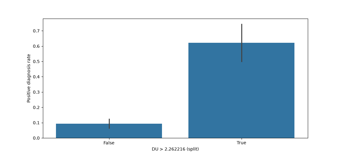
This shows that the split at 2.262216 is highly effective at separating the two classes. The right group (> 2.262216) has a 60% positivity rate compared to the left group at approximately 10%.
We then use this as a simple OneR model and make predictions for the validation set.
preds = model_val_x["DU"] > 2.262216
5.1. Evaluating the OneR Model
From this we can calculate the mean absolute error to see how off the predictions are from the actual values in the validation set:
from sklearn.metrics import mean_absolute_error
mean_absolute_error(model_val_y, preds)
0.13548387096774195
The error is relatively low, suggesting that this baseline model decent enough for a baseline.
The competition defines the metric used to evaluate submissions. I've copied the implementation from a comment in the discussion. The implementation details of this do not matter for our purposes. We just want to gauge the relative score as we go along.
def balanced_logarithmic_loss(y_true, y_pred):
    N_1 = np.sum(y_true == 1, axis=0)
    N_0 = np.sum(y_true == 0, axis=0)
    y_pred = np.maximum(np.minimum(y_pred, 1 - 1e-15), 1e-15)
    loss_numerator = (- (1/N_0) * np.sum((1 - y_true) * np.log(1-y_pred))
                      - (1/N_1) * np.sum(y_true * np.log(y_pred)))
    return loss_numerator / 2

balanced_logarithmic_loss(model_val_y.to_numpy(), preds.to_numpy())
8.588667983985555
Our local score is 8.59. When submitted to the competition (after the deadline), it had a leaderboard score of 8.56 (public) and 10.97 (private)
6. Decision Tree
After having identified the best split for the training set, we can split the data into two groups, then for each group find the next best split.
We split our training data into two groups based on the value of DU we
identified above, then find the best successive splits.
lhs = model_train["DU"] <= 2.262216
left_group = model_train[lhs]
right_group = model_train[~lhs]
left_group.shape, right_group.shape
| 396 | 59 |
| 66 | 59 |
second_level_columns = [c for c in (conts + categoricals) if c != "DU"]
left_splits = {col: min_column(left_group, col)
               for col in second_level_columns}
right_splits = {col: min_column(right_group, col)
                for col in second_level_columns}
best_left_split = get_best_split(left_splits)
best_right_split = get_best_split(right_splits)
best_left_split, best_right_split
| AB | (np.float64 (0.363205) np.float64 (0.2205227532918278)) |
| GL | (np.float64 (0.047863636) np.float64 (0.40470758822889663)) |
For our left group, column AB results in the best split and GL for
the right group. Combining the three splitting rules first splitting
by DU, then the left group by AB and the right by GL results in
a decision tree.
6.1. Using sklearn's DecisionTreeClassifier
Rather than rolling it out by hand, we can use sklearn's built-in Decision Tree classifier:
from sklearn.tree import DecisionTreeClassifier, export_graphviz

model = DecisionTreeClassifier(max_leaf_nodes=4).fit(model_train_x, model_train_y)
6.2. Visualizing the Tree
We write a procedure to visualize the created tree:
import graphviz
import re

def draw_tree(tree, df, size=10, ratio=0.6, precision=2, **kwargs):
    dot_format = export_graphviz(
        tree, out_file=None, feature_names=df.columns,
        filled=True, rounded=True, special_characters=True,
        rotate=False, precision=precision, **kwargs)
    return graphviz.Source(
        re.sub('Tree {', f'Tree {{ size={size}; ratio={ratio}',
               dot_format))
draw_tree(model, model_train_x, size=10)
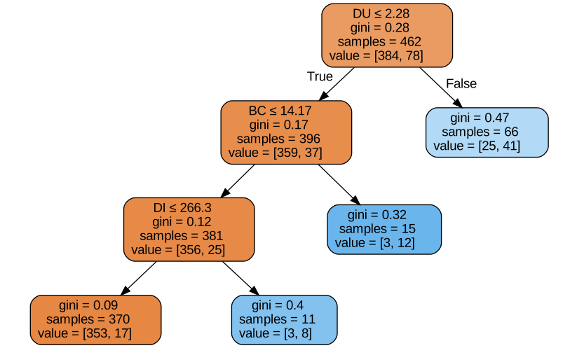
The decision tree uses a measure of impurity called the gini index. This
measures the probability that if you pick two observations from a group,
they will not have the same value for the dependent column. In the case of
perfect classification, where all observations in the group have the same
value for Class, the gini index is zero.
It is determined by subtracting the sum of squared probabilities of each class of the prediction from 1:
def gini(df, condition):
    actual = df.loc[condition, dependent]
    return 1 - actual.mean()**2 - (1-actual).mean()**2
Simulating the split at the root node above:
gini(model_train, model_train['DU'] <= 2.28), gini(model_train, model_train['DU'] > 2.28)
| np.float64 | (0.16940873380267307) | np.float64 | (0.47061524334251614) |
Like with our OneR approach, the decision tree starts with a split on DU as the best split, thought it uses a different value for the split.
The non-leaf nodes show which column was used for the split, the
split value, the gini score, the number of observations in that group
prior to the split as samples and value hints at the purity of that
group, showing how it is partitioned by the dependent variable.
6.3. Evaluating the Decision Tree
We can calculate the mean absolute error of this decision tree:
preds = model.predict(model_val_x)
mean_absolute_error(model_val_y, preds)
0.11612903225806452
And also calculate the logloss metric:
balanced_logarithmic_loss(model_val_y.to_numpy(), preds)
5.549265256402579
We see that just two additional splits have increased the accuracy on the training data considerably.
6.4. A Larger Decision Tree
We can create a bigger tree to see whether it will minimise the error further:
model = DecisionTreeClassifier(min_samples_leaf=50)
model.fit(model_train_x, model_train_y)
draw_tree(model, model_train_x, size=12)
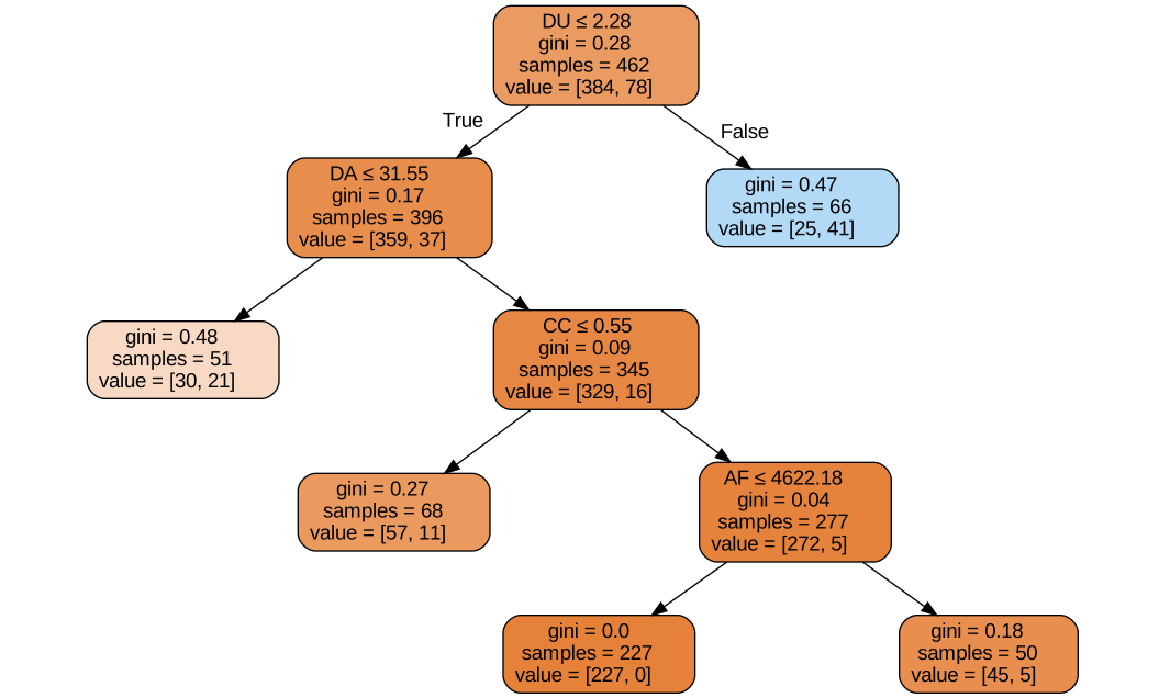
By allowing the tree to have a greater number of leaf nodes, we've allowed it to reach a grouping with a gini score of zero, which is perfect classification. However, the larger a decision tree is, the more it tends to overfit the training data and may not generalize well to the test data.
preds = model.predict(model_val_x)
mean_absolute_error(model_val_y, preds),balanced_logarithmic_loss(model_val_y.to_numpy(), preds)
| 0.12903225806451613 | np.float64 | (8.450509680016193) |
The slightly higher error than the smaller tree could hint at overfitting. When submitted to the competition, it had a score of 1.72 on the public leaderboard, an improvement over 25.97 of the OneR model.
7. Random Forests
As mentioned previously, making the decision tree bigger has it match the training data more closely, resulting in overfitting.
Instead of using bigger trees, we can use more trees. That's the insight from Leo Breiman who helped formulate the technique. By training more trees, each trained on a random uncorrelated subset of the training data and averaging their results, we get a better result. This is because the average of uncorrelated errors is close to zero.
7.1. From Scratch: Bagging Multiple Trees
To demonstrate the technique, we can train a tree on a random subset of the data:
def get_tree(proportion=0.75):
    n = len(model_train_y)
    indexes = random.choice(n, int(n * proportion))
    return DecisionTreeClassifier(min_samples_leaf=5).fit(
        model_train_x.iloc[indexes], model_train_y.iloc[indexes]
    )
Now we can train as many trees as needed and average their results:
trees = [get_tree() for _ in range(100)]
trees[:3]
| DecisionTreeClassifier | (minsamplesleaf=5) | DecisionTreeClassifier | (minsamplesleaf=5) | DecisionTreeClassifier | (minsamplesleaf=5) |
all_preds = [t.predict(model_val_x) for t in trees]
avg_preds = np.stack(all_preds).mean(axis=0)
mean_absolute_error(model_val_y, avg_preds), balanced_logarithmic_loss(model_val_y.to_numpy(), avg_preds)
The competition metric gives the best result yet of 0.42. This is the same score it received when submitted to the public leaderboard.
7.2. Using sklearn's RandomForestClassifier
sklearn's RandomForestClassifier does a similar process, but in addition
to selecting a random subset of rows, it also selects a random subset of
columns for each tree.
from sklearn.ensemble import RandomForestClassifier

rf = RandomForestClassifier(n_estimators=100, min_samples_leaf=5)
rf.fit(model_train_x, model_train_y)
preds = rf.predict(model_val_x)

mean_absolute_error(model_val_y, preds), balanced_logarithmic_loss(model_val_y.to_numpy(), preds)
| 0.06451612903225806 | np.float64 | (5.318974763205966) |
Although locally the score seems to be worse by the competition metric, on the public leaderboard it gave a score of 0.4, slightly better than the handrolled random forest approach.
7.3. Feature Importance
The random forest model can also tell us which features were most important in making the predictions:
pd.DataFrame(dict(cols=model_train_x.columns, imp=rf.feature_importances_)).plot(
    "cols", "imp", "barh", figsize=(8, 20)
)
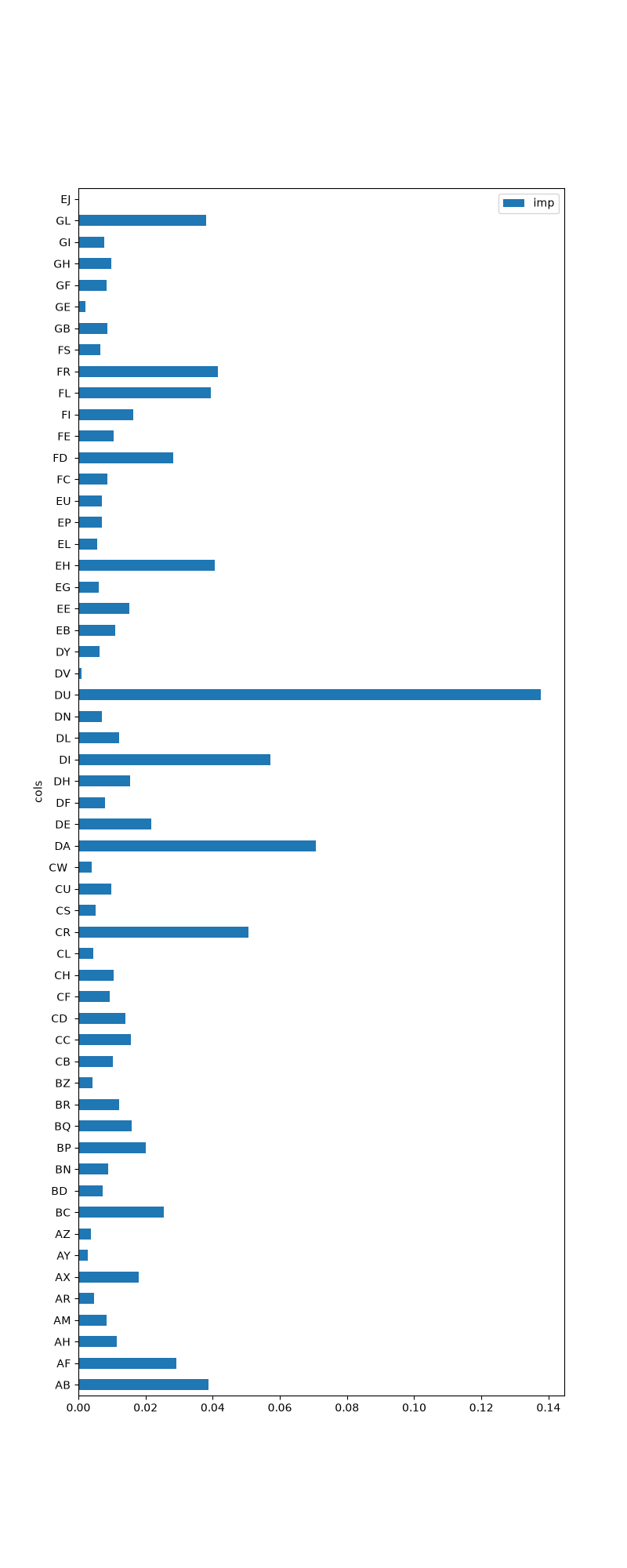
From this, we can see that DU is the column that most heavily
influences the final prediction. Since the data is anonymized, we
cannot tell what trait DU represents, but it seems to noticeably
determine the outcome.
8. Conclusion
In this notebook, we started with a very simple model, the OneR model, that makes predictions based on just a single feature of the dataset. This kind of classifier was actually found to perform competitively with other machine learning methods of the early 90s.
We improved on the OneR model by performing splits based on several features instead of one, and thus implemented a decision tree. However, the bigger decision trees are, the more they tend to overfit training data.
Next, we saw how we could improve on a single decision tree by using many trees together working in an ensemble, each making predictions and then combining their results by averaging their predictions, which gave the best score yet.
However, there's still more that can be done to get better predictions in this competition. The goal of this notebook was to demonstrate the basic techniques that apply to tabular data.
Inspired by Jeremy Howard's excellent notebook here.